In this post we'll explore Nilearn's future surface plotting capabilities through an example using seed-based resting state connectivity analysis. This is based on work done by Julia Huntenburg with whom I had the pleasure of collaborating on the 2016 Paris Brainhack.

Setting things up

We start by importing the libraries we're gonna need:

from nilearn import plotting
from nilearn import datasets
from scipy import stats
import nibabel as nb
import numpy as np
%matplotlib inline

In this example we'll use the Rockland NKI enhanced resting state dataset (Nooner et al. 2012), a dataset containing 100 subjects with ages ranging from 6 to 85 years that aims at characterizing brain development, maturation and aging.

# Retrieve the data
nki_dataset = datasets.fetch_surf_nki_enhanced(n_subjects=1)

# NKI resting state data set of one subject left hemisphere in fsaverage5 space
resting_state = nki_dataset['func_left'][0]

We'll want to define regions of interest for our analysis: for this, we'll need a brain parcellation. For this purpose, we'll use the sulcal-depth based Destrieux cortical atlas (Destrieux et al. 2009):

# Destrieux parcellation left hemisphere in fsaverage5 space
destrieux_atlas = datasets.fetch_atlas_surf_destrieux()
parcellation = nb.freesurfer.read_annot(destrieux_atlas['annot_left'])

The Destrieux parcellation is based on the Fsaverage5 (Fischl et al. 2004) surface data, so we'll go ahead and fetch that as well so as to be able to plot our atlas.

# Retrieve fsaverage data
fsaverage = datasets.fetch_surf_fsaverage5()

# Fsaverage5 left hemisphere surface mesh files
fsaverage5_pial = fsaverage['pial_left'][0]
fsaverage5_inflated = fsaverage['infl_left'][0]
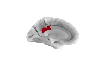
sulcal_depth_map = fsaverage['sulc_left'][0]

Last steps needed for our analysis: we'll pick a region as seed (we'll choose the dorsal posterior cingulate gyrus) and extract the time-series correspondent to it. Next, we want to calculate statistical correlation between the seed time-series and time-series of other cortical regions. For our measure of correlation, we'll use the Pearson product-moment correlation coefficient, given by $ _{X, Y} $.

# Load resting state time series and parcellation
timeseries = plotting.surf_plotting.check_surf_data(resting_state)

# Extract seed region: dorsal posterior cingulate gyrus
region = 'G_cingul-Post-dorsal'
labels = np.where(parcellation[0] == parcellation[2].index(region))[0]

# Extract time series from seed region
seed_timeseries = np.mean(timeseries[labels], axis=0)

# Calculate Pearson product-moment correlation coefficient between seed
# time series and timeseries of all cortical nodes of the hemisphere
stat_map = np.zeros(timeseries.shape[0])
for i in range(timeseries.shape[0]):
    stat_map[i] = stats.pearsonr(seed_timeseries, timeseries[i])[0]

# Re-mask previously masked nodes (medial wall)
stat_map[np.where(np.mean(timeseries, axis=1) == 0)] = 0

Plotting

Now for the actual plotting: we start by plotting the seed:

# Display ROI on surface
plotting.plot_surf_roi(fsaverage5_pial, roi_map=labels, hemi='left',
                       view='medial', bg_map=sulcal_depth_map, bg_on_data=True)
plotting.show()

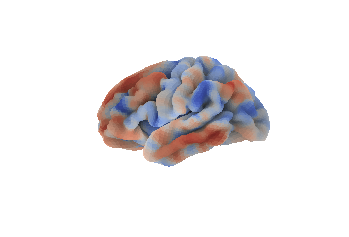
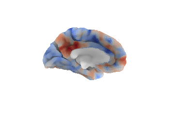
Next, we'll plot the correlation statistical map in both the lateral and medial views:

# Display unthresholded stat map in lateral and medial view
# dimmed background
plotting.plot_surf_stat_map(fsaverage5_pial, stat_map=stat_map, hemi='left',
                            bg_map=sulcal_depth_map, bg_on_data=True,
                            darkness=.5)
plotting.plot_surf_stat_map(fsaverage5_pial, stat_map=stat_map, hemi='left',
                            view='medial', bg_map=sulcal_depth_map,
                            bg_on_data=True, darkness=.5)
plotting.show()

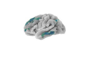
Finally, to show off Nilearn's plotting capabilities, we'll play a little with colormaps and transparency:

# Displaying a thresholded stat map with a different colormap and transparency
plotting.plot_surf_stat_map(fsaverage5_pial, stat_map=stat_map, hemi='left',
                            bg_map=sulcal_depth_map, bg_on_data=True,
                            cmap='Spectral', threshold=.6, alpha=.5)

plotting.show()

Destrieux, C., Fischl B., Dale A. M., and Halgren A. 2009. “A Sulcal Depth-Based Anatomical Parcellation of the Cerebral Cortex.” Neuroimage.

Fischl, B., A. van der Kouwe, C. Destrieux, E. Halgren, F. Ségonne, D. H. Salat, E. Busa, et al. 2004. “Automatically Parcellating the Human Cerebral Cortex.” Cerebral Cortex.

Nooner, K. B., S. J. Colcombe, R. H. Tobe, M. Mennes, M. M. Benedict, A. L. Moreno, S. Panek L. J. Brown, et al. 2012. “The NKI-Rockland Sample: A Model for Accelerating the Pace of Discovery Science in Psychiatry.” Frontiers in Neuroscience.