In this post, we'll explore different characteristics of the Brownian motion, going from the discrete to the continuous case, and finally expressing the particle's behavior in large times. This model has been the subject of various applications in different areas, like biochemistry, medical imaging and financial markets, and the domain has shown itself to be a fertile subject in mathematics, with important contributions from the likes of Paul Levy, Norbert Wiener and Albert Einstein.
Code for this post can be found here
Let \(X_i\) be a sequence of Bernoulli random variables that take the values \(-1\) and \(1\) with equal probability. We can then define the random variable \(B_n\) as:
We can show, using the central limit theorem, that \(B_n\) converges in law to a centered normal distribution of variance \(t\) when \(n\) goes to infinity. Taking this limit in a vector \((B_n(t))\) whose entries are \(B_n\) calculated at increasing times, we obtain the stochastic process \((B(t))\), that we call the Brownian movement. Its first remarkable property is that, by construction, given \(t\) bigger than \(s\):

It can also be proved that it is continuous but nowhere differentiable. Let's get an idea for what it looks like. In one dimension, for \(n=100\) and \(t=100\):
.png)
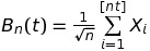
In two and three dimensions, for \(n=100\) and \(t=1000\) (the time axis is now ommited):
.png)
Quite the looker, isn't it? We'll now try a more quantitative analysis to get a feel for what's going on.
Robert Brown, the botanist after whom the process is named, first discovered it when observing the movement of pollen particules suspended in water: the random collisions of water mollecules with the particules created a very irregular movement that he was incapable of explaining. The phenomenon was later explained in detail by Einstein in a 1905 paper [1]. The model can be explained as follows: the acceleration of the particule is proportional to the force exercised by the random collisions; there's also a friction force proportional to the particle's speed (we'll call this proportionnality factor lambda). We'll ignore weight as well as buoyancy: we can get away with this because the pollen particle is really small.
We'll introduce a time interval \(\alpha\), during which the particle suffers \(N \alpha\) collisions (which we suppose to be a very large number). The collisions (which we'll identify by \(\epsilon_i\)) are supposed to be independent and identically distributed of random intensity centered at \(0\) and square integrable (of variance \(\sigma\)). We obtain the following expression then for the evolution of the particle's velocity:
Where \(Y\) is a random variable of centered gaussian distribution with variance one (which we can infer from applying the central limit theorem to the first expression). To make the notation less cluttered, we'll set \(a = -\lambda\alpha\) and \(b = \sqrt{N\sigma^2\alpha}\).
The interest of this formulation is that we can now proceed to quantitaive analysis of the position \(X_n\) and velocity \(V_n\) of a particle subject to brownian movement (\(X_n\) is just a "discrete integration" of the velocity, that is, a \(\sum\limits_{i} V_i\alpha\)).
We can now show that \(X_n\) and \(V_n\) follow gaussian distributions: even better, by exploiting the independence of \((Y_i)\), we can prove that any linear combination of \(X_n\) and \(V_n\) also follows a gaussian distribution, which allows us to conclude that \((X_n, Y_n)\) is a gaussian vector. If we note the initial position and velocity by \(x\) and \(v\) respectively, its mean is given by:
Now that we're all set up, let's see what happens when we play around with the parameters. This is a simulation for \(a = 0.5\) and \(b = 1\):
.png)
This one, for \(a = 1\) and \(b = 0.1\):
.png)
And finally, for \(a = 0.1\) and \(b = 10\):
.png)
What we see is that the term \(a\) controls the influence of the previous velocity over the next one (the "memory" of the process) and \(b\), it's degree of randomness, which goes well with our characterization of these parameters earlier (multiplying previous velocity and a random gaussian variable in the update rule, respectively). We see, in the first simulation, a random process with an upwards drift, explained by the memory of the initial velocity. In the second one, we have an almost perfect exponential, since the random character of the curve is almost suppressed by the small \(b\) value. In the final simulation, however, we have almost no memory and the process is mostly chaotic. This last one is then more likely the one that resembles the most the results that Brown found, and we can use the discrete integration process described earlier to simulate the movement of a pollen particule in the surface of a water tank based on these parameters:
So we've gotten some pretty interesting results so far for our model of Brownian movement, but you might be thinking our formulation is not yet satisfactory for a large range of problems: most systems do not behave in an organized discrete manner, weighing inputs like they were votes and then deciding which action to take at each discrete time step, but are rather complicated phenomena that are at all times being influenced by different factors in a continuous way -- or at least, like stock markets, chains of events that happen so quickly with respect to our measuring instruments and reaction times that they might as well be continuous. We can then ask ourselves if there's a rigorous mathematical way in which we can expand Brownian motion to continuous time. That's the problem we'll address in this section.
We'll take \(K\) to be the inverse of the timestep \(\alpha\). We know then, by the previous section's results, that for a fixed \(K\), \((X_t^K, Y_t^K)\) a gaussian vector. Their characteristic function \(\phi_{X_t^K, Y_t^K}\) is given by:

Where \(C\) is the covariance matrix of the position and velocity random variables. We can calculate the limits when \(K\) goes to infinity of the two expected values from the formulas we found for the expected values in the previous section:


The limit of the covariance matrix is a little bit more complicated, and so we'll omit it here: it suffices to know that it converges. We then have convergence of the characteristic function to another function \(\phi\) that's also the characteristic function of a gaussian. By Lebesgue's dominated convergence theorem, we know that \(\phi\) is continuous at zero, and so we can conclude by Levy's theorem that \((X_t^K, Y_t^K)\) converges in distribution to a gaussian vector.
In the continuous limit, velocity variance is well-behaved with respect to time, the variance of the position random variable, however, diverges. To verify this point, we'll plot histograms of \(X\) values in the continuous approximation for the times 100, 1000 and 10000, while paying attention to the axes:
.png)
.png)
.png)
We can se that the positions spread wider and wider as we increase the timescale.
This sort of behavior for the position variable, while corresponding to the idea of a free evolution of the particle, is not always desirable. More precisely, in many physical systems, the particle's a priori unbounded movement is counteracted by a force that attracts it to a center (a charged particle, a massive body). This is the sort of model we'll investigate in this section. With this goal in mind, we introduce new velocity and position random variables defined by:
Where \(D\) is called the diffusion coefficient and \(\beta\) is a strictly positive value.
The problem with this formulation is that now that the variables are coupled it is quite tricky to solve the system. A more interesting approach would be to do a spectral analysis of the recurrence matrix: for large values of \(K\), the anti-diagonal is dominated by the term \(-\beta\), that plays a regulatory role in the system, and we expect to see imaginary eigenvalues that will define an envelope curve as well as a strong oscillatory behavior. We can run a simulation of the system with large initial conditions in \(X\) and \(V\) to verify its behavior:
.png)
Besides confirming our hypothesis as we can see from the exponential envelope and sinusoidal oscillations, it is worth noting that the initial conditions become meaningless over time: the system is always brought close to the center of oscillation. What is perhaps most interesting, though, is that the system does not get arbitrarily close to the center, that is, the motion does not converge, as we can see in this simulation with zero initial condition:
.png)
[1] http://users.physik.fu-berlin.de/~kleinert/files/eins_brownian.pdf