Suppose we want to implement a biometric system in which, given a picture of a person's face taken by a camera, a software determines whether this person belongs to a predefined group of people who are allowed to perform a certain action -- this could be giving someone access to a building, or allowing them to start up a car or unlock a smartphone -- and takes a decision accordingly. One of the possible approaches to the system's design is to have a list of images of authorized users' faces and, when confronted with a new person, to analyze whether the image of their face matches with that of one of these users. This problem is known as face verification, and it's an open question that is the subject of a lot of current research in computer vision.
The diversity of situations described indicate that such a software, in order to have satisfactory performance, should be robust to most variations found in real-world images: different lighting conditions, rotation, misalignment etc.
If, on top of that, we also want to be able to easily add people to the authorized users group, it would be advantageous if our system was able to take the decision described earlier based on sparse data, that is, a small number of example pictures per user in the authorized users group. That way, the process of adding users to the group would be only a matter of taking one or two pictures of their face, which would be then added to the database.
Face Verification
Face verification can be thought of as a classification problem: given a face image space \(E\), we are trying to determine a function \(f:E\times E \rightarrow \{0, 1\}\) that associates the pair \((x_1, x_2)\) to \(0\) if it is a genuine pair (i.e. if they represent the same person) and to \(1\) if it is an impostor pair (i.e. if they represent images of different people).
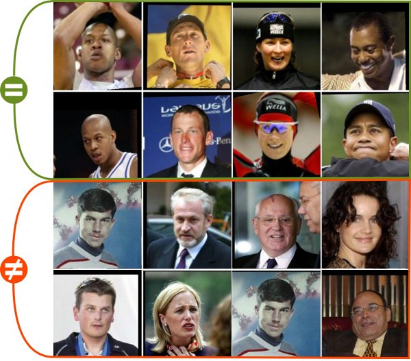
Example of genuine (top) and impostor (bottom) pairs from the LFW dataset (source: (Köstinger et al. 2012)).
Framed in the domain of machine learning, the problems becomes learning the function \(f\) from a labeled dataset comprised of genuine and impostor pairs. We'll introduce three different approaches to this problem: a simple, linear model of Exemplar Support Vector Machines (SVMs), Siamese Convolutional Neural Networks (CNNs) and the state-of-the-art identification algorithm DeepID.
Exemplar SVMs
The simplest of the three approaches is based on a method introduced by (Malisiewicz, Gupta, and Efros 2011): Exemplar SVMs. The idea is to train one linear SVM classifier, that is, a hyperplane separating our data, for each exemplar in the training set, so that we end up in each case with one positive instance and lots of negatives ones. Surprisingly, this very simple idea works really well, getting results close to the state of the art at the PASCAL VOC object classification dataset at the time of its introduction.
First, we run our training set through a Histogram of Oriented Gradients (HOG) descriptor. HOG descriptors are feature descriptors based on gradient detection: the image is divided into cells, in which all the pixels will "vote" for the preferred gradient by means of an histogram (the weight of each pixel's vote is proportional to the gradient magnitude). The resulting set of histograms is the descriptor, and it's been proven to be robust to many kinds of large-scale transformations and thus widely used in object and human detection (Dallal and Trigs 2005).
The next step is to fit a linear SVM model for each positive example in the dataset. These SVMs will take as input only that positive example and the thousands of negative ones, and will try to find the hyperplane that maximizes the margin between them in the HOG feature space. The next step is to bring all these exemplar SVMs together by means of a calibration, in which we rescale our space using the validation set so that the best examples get pulled closer to our positive -- and the worst ones, further apart (without altering their order). From there, given a new image, if we want to know whether it represents a given person, we can compute a compound score for it based on all of the person's exemplar SVMs, and decide on a threshold upon which to make our decision.
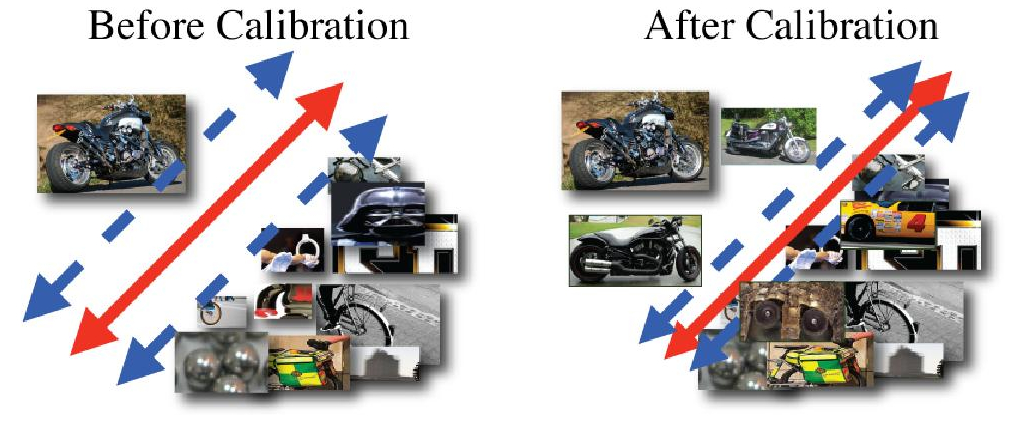
Illustration of the calibration step on an Exemplar SVM (Malisiewicz, Gupta, and Efros 2011).
Siamese CNNs
One of the ways to tackle the face verification problem is to search for a distance function such that intrapersonal distances (distances between different photos of the same person) are small and interpersonal distances (distances between photos of different people) are large. In the linear case, this is equivalent to finding a symmetric positive definite matrix \({M}\) such that, given \({x_1}\) and \({x_1}\) :
satisfies the properties above. This metric is called a Mahalanobis distance, and is has seen wide use in statistics in general and face verification and recognition in particular, specially in combination with Principal Component Analysis as in (Fan et al. 2013). The characterization of M allows is to write it as a product of another matrix and its transpose, and so \((1)\) is equivalent to:
By the manifold hypothesis, however, face space would have a manifold structure on pixel space, which cannot be adequately captured by linear transformations (Hu, Lu, and Tan 2014). One possible solution is to use a neural network to learn a function whose role is analogous to that of \({W}\) in the above example, but not restricted to linear maps. This is the option we explore in this section, and to this end we use what's called a Siamese CNNs architecture.
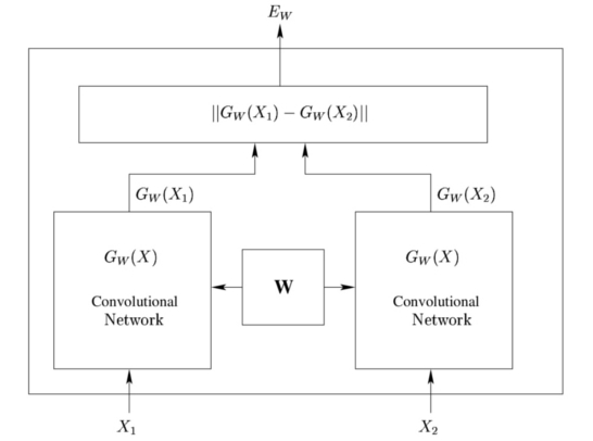
The idea of the Siamese CNNs architecure (Chopra, Hadsell, and LeCun 2005) is to train two identical CNNs that share parameters, and whose outputs are fed to an energy function that will measure how "dissimilar" they are, upon which we'll then compute our loss function. Gradient descent on this loss propagates to the two CNNs in the same way, preserving the symmetry of the problem.
Scheme of the Siamese CNNs architecture (source: (Chopra, Hadsell, and LeCun 2005)).
In our implementation, each CNN is comprised of three convolutions, all of kernel size 6x6, and computing respectively 5, 14 and 60 features, followed by a fully-connected layer that computes 40 features. Convolutions 1 and 2 are also followed by 2x2 max-pooling layers.
DeepID
Another way to tackle verification is to think of it as a subproblem of face identification, that is, the classification problem that involves assigning to each person a label: their identity. In the case of face verification, we're just trying to know if this assignment is the same for two given points in our dataset.
The jump from verification to identification can certainly be impractical: in our earlier example of biometrics, for instance, in order to prevent the entrance of undesired people, the owner of the system would ideally have to train his algorithm to recognize all seven billion people on earth. Far from this naive approach, however, lies an interesting connection that makes the exploration of this harder problem worthwhile: both problems are based on the recognition of facial features, so training a neural network to perform the hard problem of identification can in principle give very good descriptors for verification. That is the core idea behind DeepID (Sun, Xiaogang, and Xiaoou 2014), a state-of-the-art algorithm for face verification.
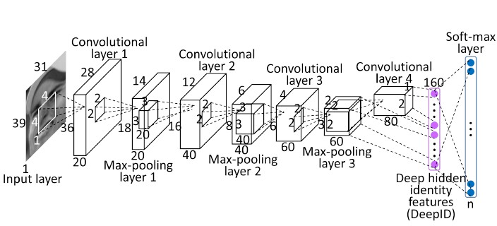
DeepID implements a CNN with four convolutional layers, of kernel sizes 4x4, 3x3, 2x2 and 2x2 and computing 20, 40, 60 and 80 features respectively. The first three layers are followed by 2x2 max-pooling, and both convolution 3 and 4 output to a fully-connected layer (named after the algorithm itself) that computes 160 features and will be used for the verification task later. Finally, for the identification task, the final layer is a softmax for classification between all the identities in the dataset.
Visualization of the DeepID architecture (source: (Sun, Xiaogang, and Xiaoou 2014)).
After training on the identification task, we can remove the softmax layer and use the fully-connected DeepID layer as a descriptor for an algorithm that will perform verification on a 160-dimensional space. In Sun's paper, the method found to have the best results was the joint-bayesian model.
Joint-bayesian models (Chen et al. 2012) the class centers \(\mu\) as well as the intra-class variations \(\epsilon\) both follow a centered gaussian distributions, whose covariance matrices \(S_\mu\) and \(S_\epsilon\) are the objects we're trying to infer from the data.
Given two observations \(x_1\) and \(x_2\), if we call \(H_I\) the hypothesis that they represent the face of the same person and \(H_E\) the hypothesis that they come from different people, we can easily see that under \(H_I\), \(x_1\) and \(x_2\) share the same class center and have independent intra-class variation, while under \(H_E\), both their class center and intra-class variation are independent. This leads us to the conclusion that the covariance between \(x_1\) and \(x_2\) under \(H_I\) and \(H_E\) are respectively:
The covariance matrices are learned jointly through Expectation-Maximization (EM), an algorithm for estimating the maximum likelihood parameter in a latent variable model through iteration of an E-step, in which we compute the distribution of the latent variables using our previous guess for the parameter, and an M-step, in which we update the parameter so as to maximize the joint distribution likelihood (for more on EM, some great notes by Andrew NG can be found here). The log likelihood here is given by \(r(x_1, x_2) = \log{\frac{P(x_1, x_2 | H_I)}{P(x_1, x_2 | H_E)}}\), and using the equation above we arrive at a closed form for it whose solution can be computed efficiently.
Chen, D., X. Cao, L. Wang, F. Wen, and Sun. J. 2012. “Bayesian Face Revisited: A Joint Formulation.” In Proc. ECCV.
Chopra, S., R. Hadsell, and Y. LeCun. 2005. “Learning a Similarity Metric Discriminatively, with Application to Face Verification.” In Proc. CVPR.
Dallal, N., and B. Trigs. 2005. “Histograms of Oriented Gradients for Human Detection.” In Proc. ICCV.
Fan, Z., M. Ni, M. Sheng, and Z. Wu. 2013. “Principal Component Analysis Integrating Mahalanobis Distance for Face Recognition.” In Proc. RVSP.
Hu, J., J. Lu, and Y.-P. Tan. 2014. “Discriminative Deep Metric Learning for Face Verification in the Wild.” In Proc. CVPR.
Köstinger, M., Hirzer, M., Wohlhart, P. and H. Bischof. 2012. “Large Scale Metric Learning from Equivalence Constraints.” In Proc. CVPR.
Malisiewicz, T., A. Gupta, and A. A. Efros. 2011. “Ensemble of Exemplar-SVMs for Object Detection and Beyond.” In Proc. ICCV.
Sun, Y., W. Xiaogang, and T. Xiaoou. 2014. “Deep Learning Face Representation from Predicting 10,000 Classes.” In Proc. CVPR.