Code for this post can be found here
Introduction
The idea of this post is to take the approach described in (Agrawal, Carreira, and Malik 2015) and implement it in a parallelized fashion. Namely, we will create a Siamese CNNs architecture for object tracking using caffe, and distribute its computations with both coarse and medium-grain parallelization using MPI (for an introduction to neural networks and CNNs, see these two posts on Christopher Olah's blog, a sketch of the principles behind Siamese CNNs can be found in my face-verification post. Finally, a great introduction to MPI and High Performance Computing in general is Frank Nielsen's book, whose preview can be found here).
Tracking
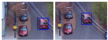
The goal of this project is to use an architecture called Siamese CNNs to solve an object tracking problem, that is, to map the location of a given object through time in video data, a central problem in areas like autonomous vehicle control and motion-capture videogames.
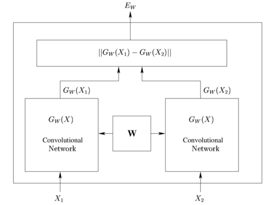
Siamese CNNs (Chopra, Hadsell, and LeCun 2005) are a model consisting of two identical CNNs that share all their weights. We can think of them as embedding two inputs into some highly structured space, where this output can then be used by some other function. Notable examples include using Siamese CNNs to determine, given two photos, whether they represent the same person (Sun, Wang, and Tang 2014) or, given two images taking consecutively by a moving vehicle, determine the translational and rotational movements that the vehicle has performed (Agrawal, Carreira, and Malik 2015).
The idea of the implementation is to train the Siamese CNNs model on evenly spaced pairs of frames in a video of an object moving, and to feed their output to another network that will try to learn the object's movement between the two frames.
A Sip of Caffe
Caffe (Jia et al. 2014) is a deep learning framework written in and interfaced with C++, created by the Berkeley Vision and Learning Center. At its core, it is based on two main objects :
Nets represent the architecture of the deep neural network : they are comprised of layers of different types (convolutional, fully-connected, dropout etc.) ;
Blobs are simply C++ arrays : the data structures being passed along the nets.
Blobs are manipulated throughout the net in forward and backward passes : forward passes denote the process in which the neural network takes some data as input and outputs a prediction, while backward passes refer to backpropagation : the comparison of this prediction with the label and the computation of the gradients of the loss function with respect to the parameters throughout the network in a backwards fashion.
Models
One of the great strengths of Caffe is the fact that its models are stored in plaintext Google Protocol Buffer (Google, n.d.) schemas : it is highly serializable and human-readable, and interfaces well with many programming languages (such as C++ and Python). Let's take a look at how to declare a convolution layer in protobuf:
layer {
  name: "conv1"
  type: "Convolution"
  bottom: "data"
  top: "conv1"
  param {
    name: "conv1_w"
    lr_mult: 1
  }
  param {
    name: "conv1_b"
    lr_mult: 2
  }
  convolution_param {
    num_output: 256
    kernel_size: 5
    stride: 1
    weight_filler {
      type: "gaussian"
      std: 0.01
    }
    bias_filler {
      type: "constant"
    }
  }
}
"Name" and "Type" are very straightforward entries : they define a name and a type for that layer. "Bottom" and "Top" define respectively the input and output of the layer. The "param" section defines rules for the parameters of the layers (weights and biases) : the "name" section will be of utmost importance in this project, since naming the parameters will allow us to share them through networks and thus realize the Siamese CNNs architecture, and "lr_mult" defines the multipliers of the learning rates for the parameters (making the biases change twice as fast as the weights tends to work well in practice).
Parallelisation
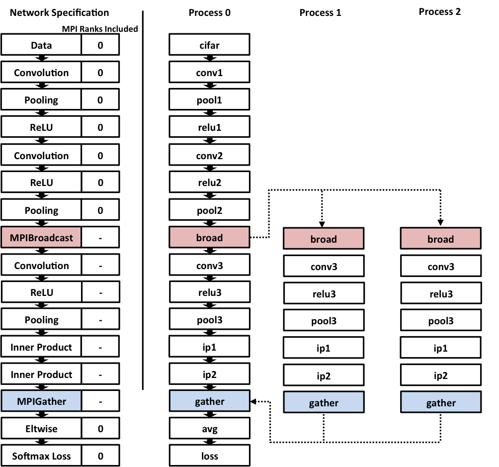
MPI-Caffe (Lee et al. 2015) is a framework built by a group at the University of Indiana to interface MPI with Caffe. By default it parallelizes all layers of the network through all nodes in the cluster : nodes can be included or excluded from computation in specific layers. Communication processes like MPIBroadcast and MPIGather are written as layers in the .protobuf file, and the framework automatically computes the equivalent expression for the gradients in the backward pass.
One of the great advantages of the model is that possibility of parallelisation is twofold:
Across Siamese Networks (medium grain): the calculations performed by each of the two Siamese CNNs can be run independently, with their results being sent back to feed the function on top;
Across Image Pairs (coarse grain): to increase the number of image pairs in each batch in training, and the speed with which they are processed, we can separate them in mini-batches that are processed across different machines in a cluster.
MNIST
The Dataset
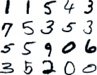
MNIST (LeCun, Cortes, and J.C. Burges 1999) is a dataset consisting of 70,000 28x28 grayscale images (split in a train and a test set in a 6:1 proportion) representing handwritten digits, with labels from 0 to 9 that stand for the digit represented by each image. The dataset is stored in the not-so-intuitive IDX file format, but we'll be using a CSV version available online in this project.
Preprocessing
For the tracking task, preprocessing was done by transforming images in the dataset by a combination of rotations and translations. Rotations were restrained to \(3°\) intervals in \([-30°, 30°]\), and translations were chosen as integers in \([-3, 3]\).
The task to be learned was posed as classification over the set of possible rotations and translations, with the loss function being the sum of the losses for rotation, x-axis translation and y-axis translation.
The Network
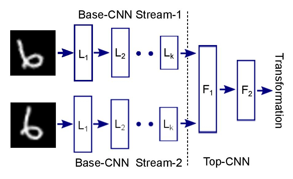
Using the nomenclature BCNN (for Base Convolutional Neural Network) for the architecture of the Siamese networks and TCNN (for Top Convolutional Neural Network) for the network that takes input from the Siamese CNNs and outputs the final prediction, the architecture used was the following:
- BCNN :
- A convolution layer, with 3x3 kernel and 96 filters, followed by ReLU nonlinearity;
- A 2x2 max-pooling layer;
- A convolution layer, with 3x3 kernel and 256 filters, followed by ReLU;
- A 2x2 max-pooling layer;
- TCNN :
- A fully-connected layer, with 500 filters, followed by ReLU nonlinearity;
- A dropout layer with 0.5 dropout;
- Three separate fully-connected layers, with 41, 13 and 13 outputs respectively (matching number of rotation, x translation and y translation classes);
- A softmax layer with logistic loss (with equal weights for each of the three predictions).
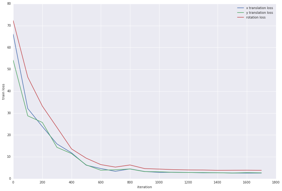
Results
The network was trained using batches of 64 image pairs, with a base learning rate of \(10^{-7}\) and inverse decay with \(\gamma = 0.1\) and \(\text{power}=0.75\). The network seemed to converge after about 1000 iterations, to an accuracy of about \(3\%\)for the rotation prediction and \(14\%\) for the x and y translation predictions (about 1.25 times better than random guessing for the rotation and 2 times better for the translations).
Coarse-Grain Parallelization
The simplest way to parallelize the program is to run multiple training batches on different nodes, as in the scheme below:
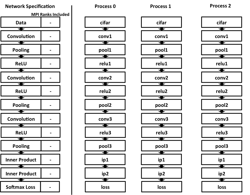
In this case, we're gaining a speedup in the Gustafson sense, that is, as we raise the number of processors, we also raise the size of the data we can compute in a given time. The speedup expression is then given by:
\[\text{speedup}_{\text{Gustafson}}(P) = \alpha_{seq} + P(1 - \alpha_{seq}) \]
where P is the number of processors and \(\alpha_{seq}\) is the proportion of the code that's not being parallelized. Seeing as in this scheme the whole network is being parallelized, we have:
\[\alpha_{seq} \approx 0 \Rightarrow \text{speedup}_{\text{Gustafson}}(P) \approx P \]
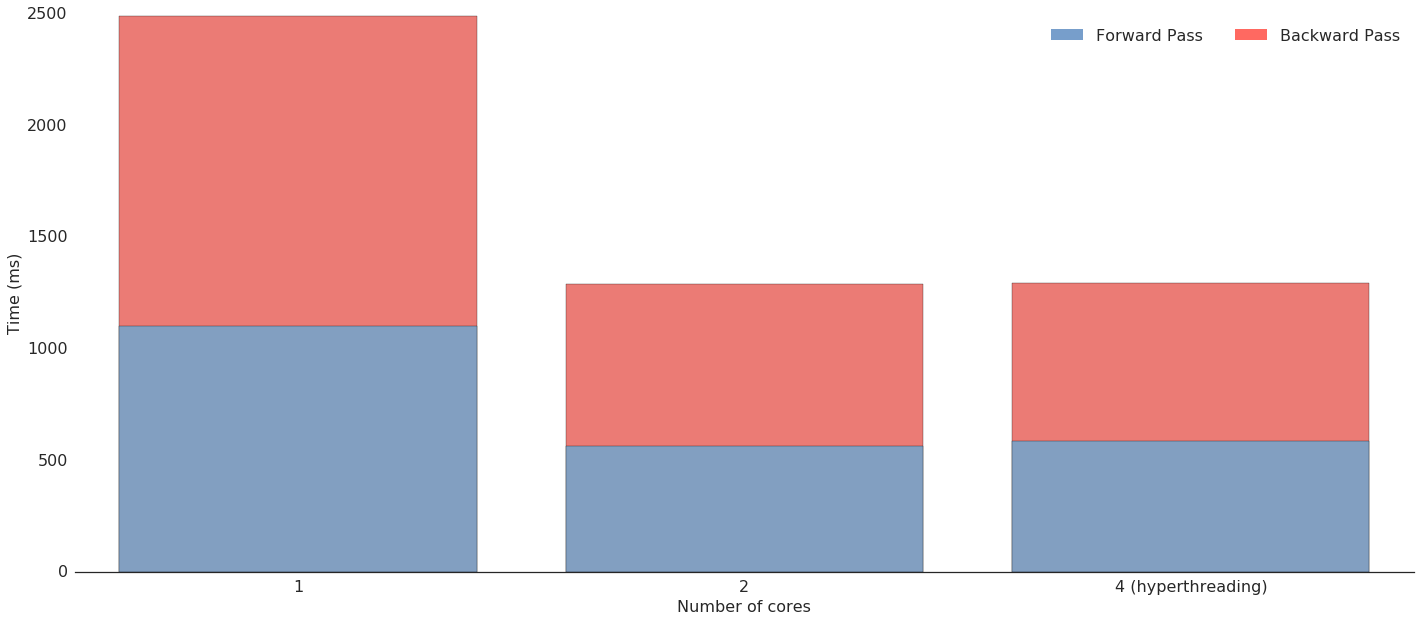
Let's see how this fares in practice. In the figure below, we find a comparison of running times for the forward and backward passes in the network for one, two and four cores, the four core option using hyperthreading. What we find is that the two core case follows Gustafson's law closely, with a speedup coefficient of \(1.93\). In the four core case, however, performance is no better than with two cores, which probably means that hyperthreading is making no difference for this task.
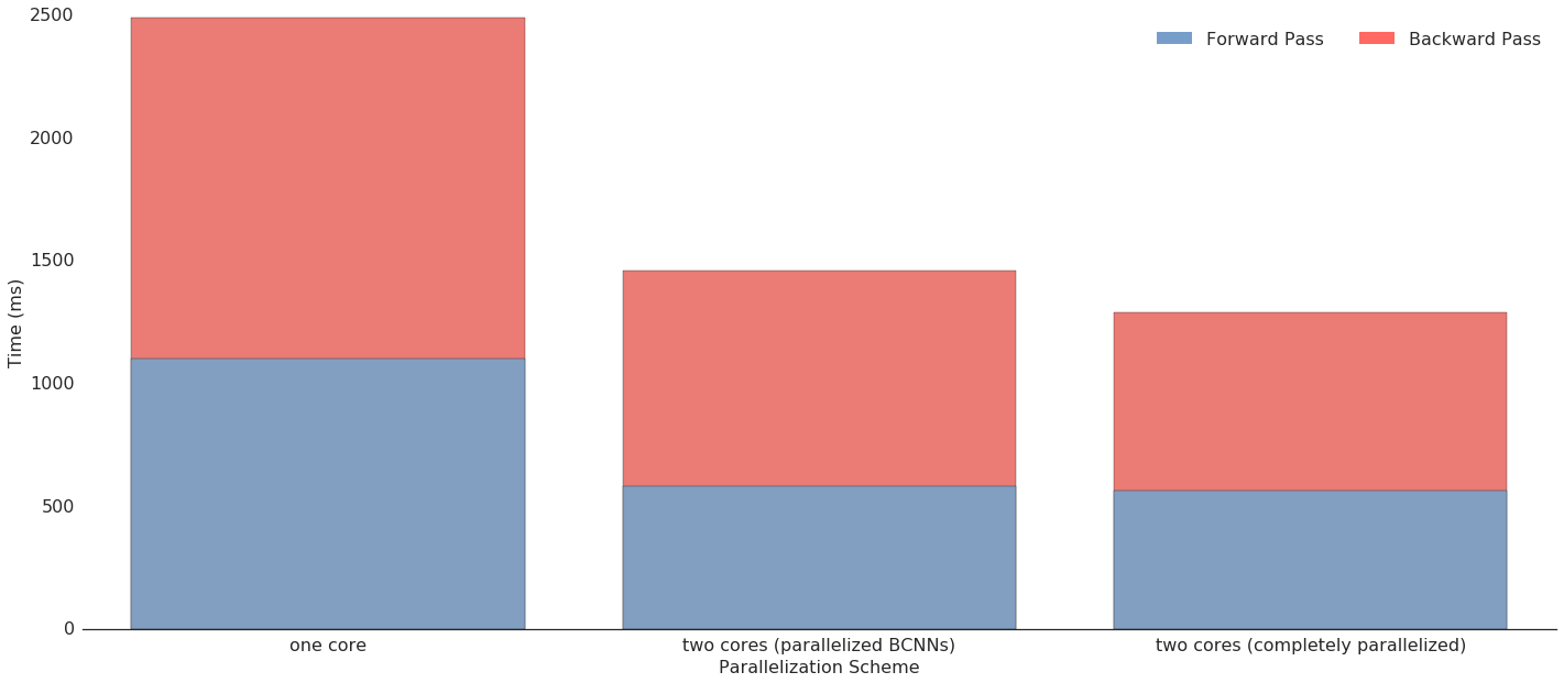
Medium-Grain Parallelization
The interest of the Siamese CNNs architecture, however, is the possibility of parallelization on a lower level : we can distribute the two BCNN streams to two different nodes in the cluster, and then gather their results to perform the computations on the TCNN. Results are shown in the figure below: we can see that performance is almost as good as in the completely parallelized scheme, which confirms our knowledge that the convolutional layers are by far the most computationally-intensive ones, so that the BCNN accounts for most of the computations in the network. We can also see that the difference between these two parallelization schemes lies almost entirely in the backward pass: we can hypothesize that this is due to increased difficulty in computing the gradient through the gather and broadcast layers in the Medium-Grain scheme.
Agrawal, P., J. Carreira, and J. Malik. 2015. “Learning to See by Moving.” ArXiv Preprint.
Chopra, S., R. Hadsell, and Y. LeCun. 2005. “Learning a Similarity Metric Discriminatively, with Application to Face Verification.” In Proc. CVPR.
Google. n.d. “Protocol Buffers.” http://code.google.com/apis/protocolbuffers/.
Jia, Y., E. Shelhamer, J. Donahue, S. Karayev, J. Long, R. Girshick, S. Guadarrama, and T. Darrell. 2014. “Caffe: Convolutional Architecture for Fast Feature Embedding.” ACM Multimedia Open Source.
LeCun, Y., C. Cortes, and C. J.C. Burges. 1999. “The MNIST Database of Handwritten Digits.” Http://yann.lecun.com/exdb/mnist.
Lee, Stefan, Senthil Purushwalkam, Michael Cogswell, David J. Crandall, and Dhruv Batra. 2015. “Why M Heads Are Better Than One: Training a Diverse Ensemble of Deep Networks.” ArXiv. http://arxiv.org/abs/1511.06314.
Mei, X. and Porikli, F. 2008. “Joint Tracking and Video Registration by Factorial Hidden Markov Models” IEEE International Conference on Acoustics, Speech and Signal Processing (ICASSP).
Sun, Y., X. Wang, and X. Tang. 2014. “Deep Learning Face Representation by Joint Identification-Verification.” Proc. NIPS.